In valuation, the name of the game is expected future cash flows. It’s not about the past, it’s about the future. So in trying to estimate the value of an asset, an intelligent cash flow projection is critical. And it’s rife with pitfalls.
As we know, there’s a myriad of destructive biases and ideas that can lead a good valuation model astray. I won’t unpack them all here.
There are some key historical statistics to help us avoid many of those kinds of traps.
In his fascinating and in-depth book on stock market statistics and reversion to the mean by Michael Mauboussin called The Base Rate Book, Mauboussin dives into arguably the most important inputs for a good cash flow projection— including revenue and operating profit/margin.
This book is not light reading, especially if you are not well versed in high level mathematics and statistics; it took me most of a morning and a fresh cup of coffee to unpack just the revenue and operating profit part.
But it’s those sections that we will discuss, as studying their history of behavior (depending on stock market sector) lead to better cash flow projections and thus better valuation estimates for a DCF.
Introduction to Reversion to the Mean
One of the building blocks of building a DCF (Discounted Cash Flow) Model in the first place is the idea of reversion to the mean.
In the stock market, stocks can sometimes trade at market values which are separated from their true intrinsic value (the value of the underlying business).
Over the long term, a stock’s price will tend to “revert to the mean”; in other words the price will eventually catch up with its true intrinsic value where it belongs.
There’s two main ways to make excess (market-beating) returns in the stock market over the very long term:
- Buy stocks trading below their intrinsic value and profit as they revert to the mean
- Buy stocks trading at their intrinsic value, and earn a compounding rate of return that exceeds the underlying company’s rate of return on capital invested (versus their cost of capital)
If that’s a mouthful to digest, that’s okay. We’re going to focus on the reversion to the mean part as we discuss the concept further and how it applies to an intelligent cash flow projection.
The Mathematics of Reversion to the Mean
But reversion to the mean doesn’t just apply to stock prices and a company’s intrinsic value. It also applies to all statistics, at least with those where reversion to the mean is a factor.
A “mean” is simply an average of a group of numbers.
Reversion to the mean states that if you take a group of numbers, and calculate the future probability on the next dataset of numbers, there will be a likelihood that future probabilities settle back down to the average, or “mean”.
Take coin flipping as an example.
Whether you want to believe it or not, the probability of flipping a balanced coin and returns heads or tails is exactly 50-50, or 50% for heads and 50% for tails.
Let’s say we took a group of 100 coin flippers, and recorded their flips over 24 flips.
With enough flips to allow us to record a dataset that is large enough to be significant (large enough “sample size”), we will see a wide range of results.
Just because the odds are 50-50 doesn’t mean that every flipper will end up with 12 heads and 12 tails. There is an element of luck involved.
But with a large enough sample size, we should see a “mean”, or average, of heads-and-tails percentages very close to 50%.
There will be some “outliers”, or flippers who got extremely lucky or unlucky to have many heads or many tails, but over the dataset—there’s probably a mean close to 50%.
Reversion to the mean says that future results for these flippers will trend close to that mean of 50%.
In fact, if we had the flippers do 240 flips or 2400 flips, there’s likely to be less “lucky” or “unlucky” streaks sustained since the real probability of either outcome is exactly 50%.
Whether a flipper had 80% tails or 50% tails over 24 flips, both are likely to have 50% odds in the flips to follow.
As a result, the longer we have those flippers flip, the closer to 50% their final results will converge to.
That is reversion to the mean.
Reversion to the Mean in Business
We also tend to see reversion to the mean in the business world.
One of the most commonly used applications in this is with profit margins.
A profit margin simply compares a company’s profits to its revenues. The formula is profit divided by revenue. Higher profit margins need less revenues to grow, and so all else equal, higher profit margins lead to higher/faster growth.
But in the real world, all else is not equal. High profit margins also tend to attract sharks, and as more competitors enter a market this tends to drive profit margins down.
In other words, there’s an average profitability throughout the business world and stock market.
Because companies constantly compete and seek higher profitability, they will tend to move into markets where there is higher profitability (profit margins). As these forces bring profitability down, the profitability of an industry or market will revert to the mean, or the mean of all of the profitability margins anyone could invest or start a business in.
That’s at least what conventional wisdom and business schools tell us.
Mauboussin found that:
- Not every business statistic reverts to the mean
- Not every business statistic reverts to the mean in the same way, some revert more than others
- Not every industry reverts to the mean with a certain business statistic in the same way
Mauboussin studied several key business and stock market statistics in his Base Rate book; I’m going to focus on two that are among the most important to a cash flow projection for a DCF, at least on the NOPAT side (before factoring in investment of working capital and capex).
Note that I’m choosing these two metrics based on my own personal opinion, feel free to take what you find valuable from this research and apply it to your own thoughts and opinions.
Key DCF Valuation Model Inputs
When modeling a company’s expected future cash flows, you can take many different paths.
One approach which I’ve used in the past and like to use for certain companies is a backwards, top down kind of approach.
In this one, you take a estimate for free cash flow per share based on historical data, and then project a growth rate based on a combination of business, industry, and macro factors.
For the free cash flow side, you can start with a simple Cash From Operations and Subtract Capital Expenditures (Capex), or calculate it starting with the Income Statement in various ways.
For the growth estimate, you can look at a variety of key factors especially a company’s moat and industry positioning as well as the prospects of the industry it is in and the success of the company so far.
By combining your estimates for free cash flow per share and growth and inputting them into a DCF valuation spreadsheet, you get a cash flow projection which can be used to estimate an intrinsic value for a business.
A second approach which I’ve seen podcast co-host Dave Ahern use a lot lately, and one I find attractive especially when using reversion to mean in valuation is through separate forecasts of key line-items:
- Revenue and revenue growth
- Operating Income and Operating Margin
- Corporate Tax Rate
- Investment of Working Capital and Capex
I particularly like this approach when it’s possible that a company’s latest historical financial results are temporarily unfavorable due to suppressed margins that are likely to bounce back (revert to the mean).
No company grows without challenges, even great ones, and so if we can identify these who temporarily stumble we can find some great deals in the stock market.
Because Mauboussin’s book had groundbreaking results on revenue growth and operating margin, we will focus on these findings for the rest of this post. I encourage also learning about and determining capital investment of working capital and capex to fully complete your DCF model, after you finish reading this post.
Interpreting the Base Rate Report
Just like we had to make some basic definitions of statistics and mathematics to understand reversion to the mean, we’ll need a few more advanced defitions to understand Mauboussin’s report.
I’ll summarize as best as I can, but I highly encourage reading through the report yourself and using my summary as a supplement. I can’t possibly cover every key part of his report in my summary, and that’s what makes it a summary. There’s so much good stuff there, so read it too.
First we need to understand the following terms:
- Correlation Coefficient = “r”
- Standard Deviation
- Coefficient of Variation
Don’t worry, I didn’t know or couldn’t remember what these terms meant so I had to go back and study them; hopefully you get a simplified 101 explanation here.
Correlation Coefficient
Correlation coefficient, or in Mauboussin’s report “r”, is basically how likely a statistic is to revert to the mean.
A statistic with an “r” of 0 would revert to the mean perfectly, an “r” of 1 has no reversion to the mean so there’s probably not much luck or randomness in future results.
Remember that in our previous example, over enough coin flips the results revert to the mean, so the “r” for coin flipping is 0.
Basically, a statistic’s “r” depends on how much skill or how much luck is involved.
I love the way he describes it by comparing sports.
The game of basketball is inherently more reliant on skill, while the game of hockey is inherently more reliant on luck.
Logically, we can confirm this in several ways—a hockey game has many less goals and any one lucky bounce can determine a goal. Contrast that to basketball with dozens of shots (field goals) and much higher scores in any single game. There’s also many less lucky bounces in a basketball game than a hockey game.
In the report Mauboussin shared a chart where the NBA (basketball) had an “r” closer to 0.80 and the NHL (hockey) and one that appeared to be closer to 0.55.
So skill is still involved, but it appears that helps more in the NBA than NFL based on the data.
Standard Deviation
Next is standard deviation. What this measures is the likely range of all outcomes.
The example of human height is a great way to understand standard deviation. The average height for an adult male is about 5’9” (at least in the United States).
There are some outliers, you have a few giants above 7” and a few vertically challenged below 5”. But those outliers are few, most males are close to the 5’9” average with the probability of you being much taller or shorter than this exponentially decreasing over time.
If you were to plot the distribution of men’s height in a chart, you would get something like a bell curve, where the top most point is the “mean”, in this case 5’9”.
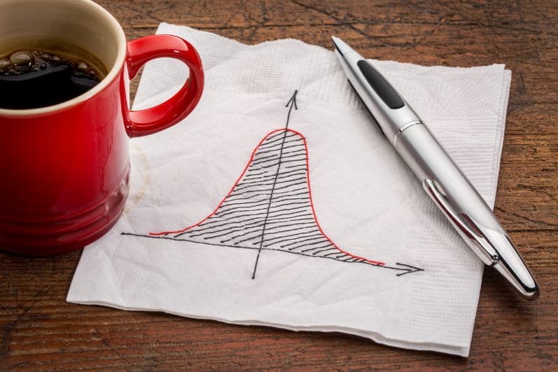
Each statistic will have a different shaped bell curve. Some will be skinnier and some will be fatter than others.
What we’re trying to do when studying reversion to the mean and standard deviation is to estimate where the majority of cases lie.
For our purposes, and I’m not an expert here, but I believe a standard deviation of “1” (one) represents 68% of the datapoints. Picture that visually as (roughly):
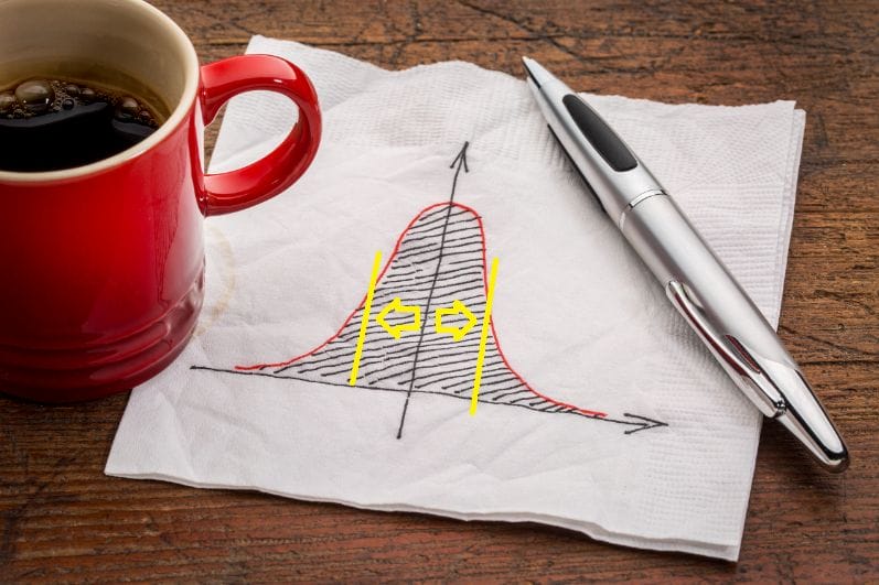
So let’s say that 68% of adult males had a height of 5’7” – 5’11”. Each of those heights are 2 inches away from 5’9”. Since our mean is 5’9” and 68% = 1 standard deviation are each 2 inches away, a standard deviation of 1 in this sample size is 2 inches.
Think of it this way.
The mean tells you where the average lies. The standard deviation tells you where the majority lies.
You take the standard deviation (of 1) and add and subtract it from the mean, and you get your answer to where the majority (68% of cases) lies.
Explaining our example one more time—the mean is 5’9”. Say the standard deviation of 1 for adult male height is 2 inches. So, 68% of adult males would be somewhere between 2 inches below and 2 inches above our mean = 5’7” – 5’11”.
Coefficient of Variation
This one is less important for our simplified purposes but if you’re going to read Mauboussin’s report you should get this definition under your belt too.
The coefficient of variation is trying to explain how wide the standard deviation is.
For example, human height doesn’t have much standard variation. A difference of 2 inches isn’t much. Contrast that to average net worth. You have some people with $50k in Net Worth, and some with $50 million. That’s a huge difference, a huge standard deviation.
What the coefficient of variation does is allow us to compare each of those even though we are measuring height in inches and net worth in dollars.
The formula for the coefficient of variation is one standard deviation divided by the mean.
So for our height example, that would be:
= (2 inches) / 5’ 9”
= 2 inches / 69 inches
= 0.029
But let’s say the average net worth is $55k, but our standard deviation is something like $100k, since there’s a lot of very rich people pushing up the average.
Our coefficient of variation for this wealth example would be:
= 100,000 / 55,000
=1.818
The higher the coefficient of variation, the higher the deviation is from the average. Height at 0.029 had a small variation, as most adult males sat within 2 inches of the mean.
But our wealth example had 1.818 of variation, which means there was a huge range in one standard deviation (-$45k to $155k). The majority of people (68%) sat somewhere in this wide variation.
With our coefficient we can compare how wide a statistic’s standard deviation is, which lets us compare the variability in the statistic compared to another.
Reversion to the Mean in Revenue
Remember that we have two main parts for the NOPAT of our cash flow projection, revenue growth and operating margin (taxes are an easier estimate).
Let’s start with revenue growth first.
Mauboussin examined an entire universe of stocks from 1950-2015 and ranked them based on Sales Size, starting with a group at ($0 – $325 million) all the way to a group of $50 billion+. These sales numbers were inflation adjusted.
I found this fascinating…
The “r” for 1 year revenue growth, 3 year revenue growth, and 5 year revenue growth was 0.30, 0.17, and 0.19 respectively.
Remember that the lower the “r”, the more luck involved.
This means that revenue growth historically had a lot of luck involved especially in a 3 year and 5 year period, and so it had much more reversion to the mean.
Another fascinating tidbit…
The median sales growth declined as total company sales got bigger and bigger. Check out Mauboussin’s chart for the whole story, but I’d like to highlight the 10y revenue growth numbers for mean and standard deviation:
- $0-$325m: Mean = 12.6% (Median = 9.8%); Std Deviation = 12%
- $325m-$700m: Mean = 7.4% (Median = 6.7%); Std Dev = 7.0%
- $700m-$1250m: Mean = 6.2% (Median = 5.7%); StDev = 7.0%
- $1.25B-$2.0B: Mean = 5.7% (Median = 5.1%); Std Dev = 6.6%
- $2B – $3B: Mean = 5.1% (Median = 4.5%); Std Deviation = 6.0%
- $3B-$4.5B: Mean = 4.4% (Median = 4.1%); Std Deviation = 5.7%
- $4.5B-$7B: Mean = 3.9% (Median = 3.7%); Std Deviation = 6.0%
- $7B-$12B: Mean = 3.3% (Median = 3.2%); Std Deviation = 6.0%
- $12B-$25B: Mean = 2.9% (Median = 2.7%); Std Dev = 6.1%
- $25B+: Mean = 1.7% (Median = 1.8%); Std Deviation = 6.1%
- $50B+: Mean = 0.8% (Median = 1.1%); Std Deviation = 5.8%
It’s incredible to me how much lower the median revenue growth got the higher the total sales for the company. This means that the higher in total sales you go, the more low revenue growth companies (statistically) there are!
But, notice how high the standard deviation stayed; it was basically 6% or 7% for almost every group.
That means that there were a lot of companies somewhere within a 12% – 14% range of results, which is a huge difference!
Take the $12B – $25B in sales group as an example.
If the mean was 2.9%, but the std deviation was 6.1%, then the majority (68%) of companies in this range had revenue growth rates around anywhere between plus or minus 6.1% of 2.9%, or -3.2% to 9%!!
Talk about a wide range in valuation results!
So to wrap up thoughts on revenue growth, if there’s lots of reversion to the mean (lots of luck involved), and the range of possible outcomes is so large, then a cash flow projection based solely on a revenue estimate is practically worthless!
Even historical revenue growth rates don’t seem very helpful here, especially if they fall outside of the standard deviation set based on their sales growth side.
It will probably pay to project revenues close to their median based on sales size, but realize that there’s a huge potential variability in that final result. And there’s lots of reversion to the mean involved.
Reversion to the Mean in Operating Margin
Where revenue growth had so much luck involved, I was surprised to find out that operating margin had almost the exact opposite effect!
In other words, companies with high operating margin were likely to sustain high margins, while companies with high revenue growth were not likely to sustain that growth.
Sorry, spoiler alert.
You really should read the entire section Mauboussin did on Operating Profit Margin, but I’ll just pull a key relevant statistics for my application.
Looking at the operating margin for eight sectors over 1950-2015, Mauboussin found the following 5-year correlation coefficients “r” (I inputted his standard deviation result for easier understanding):
- Consumer Staples = 0.83 – 0.95
- Health Care = 0.64 – 0.84
- Consumer Discretionary = 0.69 – 0.81
- Industrials = 0.63 – 0.81
- Telecommunications = 0.40 – 0.86
- Materials = 0.49 – 0.75
- Information Technology = 0.49 – 0.75
- Energy = 0.48 – 0.76
A lot of this is actually intuitive.
Energy companies are subject to huge cyclical and commodity cycles, swings, and boom/bust periods. So their results, and profit margins, swing wildly from year to year depending on those outside factors. That means their results depend on a lot of luck, and have large reversion to the mean, over a 5 year period.
Consumer staples is a pretty stable market; people need to buy these products regardless of economic conditions, which is why they are called staples. So these companies tend to sustain their profit margins, which means companies with high profit margins in their industry are likely to continue to earn those while those with lower profit margins are less likely to increase them from reversion to the mean.
The strong get stronger in those industries while the weak stay weaker (or disappear).
Investor Takeaway
I hope these findings were as eye opening to you as they were to me.
How you apply them all depends on what flavor of a DCF Valuation Model you implement. I don’t think one model is better than the other, you should have multiple tools for multiple applications when trying to project future free cash flows.
My biggest takeaways from this piece were:
- A revenue growth estimate way above their expected standard deviation of results based on their sales size is probably ill-advised
- Historical revenue growth is probably much less useful as an estimate than most people (myself included) realize
- Don’t depend on operating margin expansion especially in a high “r” sector
- Look for businesses with high operating margins in sectors where this could reasonably continue
One word of caution, I’ll add it as a “note to my future self”:
Be careful of making absolute conclusions based on the sector data from the Base Rate report. For example, many telecommunications stocks used to be THE growth stocks of their day. Many IT companies of today could behave like the industrials of yesterday. Don’t overgeneralize.
At the end of the day, it’s the same theme Dave and I have been harping on.
Valuation and thus a cash flow projection really depends on the business, and is a business-by-business practice. Develop a circle of competence, study the business deeply, and only then make bolder and riskier cash flow projections and investments.
