Value-at-Risk (VAR) is a critical concept for risk and portfolio management which is often taught during CFA level II and level III. Value-at-Risk is a measure of the minimum loss expected in either dollar or percentage terms as it relates to the portfolio value. VAR is measured both over a period of time (ex. 1 year) and also at a confidence level for which losses will not exceed an amount or percentage (ex. 95% confidence).

The end goal of doing a VAR calculation is being able to make a statement such as there is 5% probability in any given year that the loss of the portfolio will exceed $100,000 and a 95% probability the loss will be less than that. This article will teach analysts and investors how to calculate value-at-risk, convert VAR for different time periods and confidence levels, as well as walk readers through examples with a sample portfolio. For our ongoing example throughout this reading, we will look at a hypothetical $1 million portfolio with annual expected returns of 10% and a standard deviation of 6%.
Value-at-Risk Formula
The value-at-risk formula starts by looking at the expected return of the portfolio over the time period (ex. 10%) and then subtracts off the standard deviation of the portfolio (the risk) which is multiplied by the Z-Score of the confidence interval we are looking to analyze. The Z-Score is a statistics term for a normal distribution which we will discuss in more detail next, but there are common Z-Scores that can be remembered for each confidence interval.
Value-at-Risk (%) = [Expected Return – (St. Dev of Portfolio x Z-score of Confidence Interval)]
= [(10% – (6% x 1.65)]
= 10% – 9.9%
= 0.1%
The above formula will give the value-at-risk in percentage terms. For example, this formula would spit off the calculation that at a 95% confidence level, portfolio returns will be greater than 0.1% in a one year period and a 5% probability they will be less than 0.1%. To get this amount into dollar terms, we simply multiply the outcome of this formula by the value of the portfolio, as can be seen below. The VAR formula can then be manipulated algebraically to solve for any of the independent variables in an analysis.
Value-at-Risk ($) = Value-at-Risk (%) x Portfolio Value ($)
= 0.1% x $1,000,000
= $1,000
Confidence Intervals for Value-at-Risk
The confidence intervals represents how sure an analyst wants to be that portfolio losses will not exceed a certain percentage or dollar value of the portfolio. The Z-Score is a statistical measure for a normal distribution curve of the number of standard deviations (#) away from the expected portfolio return (the average) that a certain percentage of calculated returns will fall under. Assuming a normal distribution curve as can be seen below, the percent of portfolio return scenarios which fall outside specific standard deviations away from the average portfolio return stays constant.
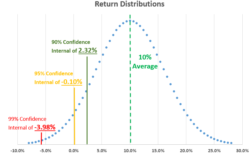
Because this is a risk analysis (and not an upside return analysis), we are only concerned about the lower part of the normal distribution curve. As can be seen below, a 90% confidence level (could also be referred to as 10% VAR) will be 1.28 standard deviations away from the average expected portfolio return. At a 95% confidence level, we are 1.65 standard deviations away from the average. And, at 99% confidence level, we are 2.33 standard deviations away from the average. As mentioned previously, these Z-Scores or standard deviations stay constant under a normal distribution.
Confidence Levels (One-tail):
90% Confidence (10% VAR) = 1.28 St. Dev
95% Confidence (5% VAR) = 1.65 St. Dev
99% Confidence (1% VAR) = 2.33 St. Dev
Cautious Side Note: Value-at-risk is a good estimation of risk but is far from perfect and has significant flaws in assuming that return distributions are normal. Fans of the movie Margin Call, about the 2008 financial crisis, would recall the opening scene where analysts are huddled around a computer anxiously talking about recent data in the markets falling outside their model predictions. This conversation signifies that the return data was not normally distributed having fat or long downside tail ends which were not properly taken into account when calculating risk of the portfolio.
Time Conversion for Value-at-Risk
Often we have data for average returns and standard deviations that have been collected over a specific period of time. To make this data more relevant and to answer various risk management questions, we can convert this data for different time periods. The mathematics to make this conversion are based off the idea that standard deviation of returns increase/decrease with the square root of time. When dealing with investment portfolios, some of the common time periods to know off hand are that there are 20 trading days in a month, 250 trading days in a year, and of course, 12 months in a year.
In our example, we started with data that was based on annual return figures of 10% and a standard deviation of 6%. To convert this into a monthly value at risk, we will need to 1) adjust the return by using simple division, 2) convert the standard deviation by dividing by the square root of time, and 3) feeding it back into the VAR equation. In this conversion, we are going from annual to monthly (getting smaller) so we are using division. If one was converting to a longer time period, we would use multiplication in its place.
Example for VAR Time Conversion: For a $1 million portfolio with annual expected returns of 10% and a standard deviation of 6%, what would the value-at-risk be on a monthly basis at a 95% confidence level?
- Convert the return from annual to monthly using simple division or multiplication
Returnmonthly = Returnannual / 12
= 10% / 12
= 0.8333%
- Convert the standard deviation by dividing by the square root of time, in our example 12 months.
St. Devmonthly = St. Devannual / 12^(1/2)
= 6% / 3.4641
= 1.7321%
- Place the new converted metrics back through the VAR equation.
VAR ($) = Return – (St. Dev x Z-score) x Portfolio $
= 0.8333% – (1.7321% x 1.65) x $1,000,0
= (0.8333% – 2.8580%) x $1,000,000
= -2.0247% x $1,000,000
= -$20,247
As can be seen from the loss value of the worst 5% converted monthly VAR, risk has increased due to the new monthly returns being lower proportionately compared to risk which has only decreased by the square root of time. The other way to think about this disproportionate relationship with the value-at-risk being higher over a short time is that long-term returns and risk have not had time to average out yet. This is also why long-term investing leads to better returns in investing!
Historical Value-at-Risk
The historical method to determine value-at-risk looks at actual historical results for the portfolio rather than using the average and standard deviation to graph a normal distribution and make mathematical calculations. In a historical VAR analysis, actual historical results are arranged in order from worst to best and then the lowest historical monthly returns are used to determine what risk to expect.
For example, if asked for 5% VAR (95% confidence level) and given 120 months of data, then month six (120 months x 5%) when the historical returns are arranged in order would be the 5% threshold of returns to expect. Counting up when arranged in order to the sixth worst value would give you the historical value-at-risk.
Takeaway on Value-at-Risk
Value-at-Risk (VAR) is a critical concept for risk and portfolio management which is often taught during CFA level II and level III. Value-at-Risk is a measure of the minimum loss expected in either dollar or percentage terms as it relates to the portfolio value. The VAR metric is a good estimation of risk but is far from perfect with outliers in data and long tails in the distribution causing potential. Knowing the value-at-risk equation well, analysts can do time conversions and solve for different variables in the VAR equation.
